Computer Vision Against Construction Site Theft: What Real Deployments Show

Computer vision on a construction site is not a camera with a clever label. It is a classification model running against a defined visual field, tuned to a finite set of events, embedded in a chain of decisions that ends with someone responding within a stated number of minutes.

That definition matters because most of what gets sold under the heading "AI on site" is something else. It is recorded footage with motion detection, accessible from a phone, sold on the promise that the operator will look at the right clip at the right moment. Recorded footage is forensic. It tells the loss adjuster what happened. It does not interrupt the theft. The distinction between forensic recording and active deterrence is the distinction between insurance documentation and security technology, and it is the first thing an operator has to settle before any vendor conversation becomes productive.

What follows is a description of how serious deployments behave, what they detect, what they miss, and how the cost case actually closes. The patterns described here are drawn from active sites, not from product brochures.

What computer vision detects, and what it does not

A modern detection model on a fixed or mobile camera mast distinguishes between a small number of object classes with high reliability and a larger number of behavioural patterns with declining reliability. The classes that work are persons, vehicles, and a defined set of equipment categories. The behaviours that work are presence in a zone, movement direction, loitering above a time threshold, and approach to a marked perimeter. These detections, in good light and clean weather, run above ninety percent precision on properly trained models. NIST and the relevant test bodies publish ranges in this region for comparable industrial classifiers, and our own field data sits inside that band.

The detections that do not work, or that work only with high false-positive rates, are the ones vendors describe in marketing material. Intent recognition is one. A model cannot tell whether a person walking past a stack of copper is a thief or a passing pedestrian. It can tell that the person stopped, that the person bent over, that the person carried something away. Three behavioural signals chained together approximate intent. Single signals do not. Operators who buy systems that promise intent recognition end up turning the alerts off within six weeks, because the false-positive rate destroys the operator's room to respond.

The second class of detections that does not work reliably is fine-grained tool identification at distance. The model can see that something was carried. It often cannot say whether it was a drill or a thermos. This matters in the legal sequel of a theft, because the chain of evidence requires identification, not suggestion. The serious deployments compensate for this by combining wide-area detection with a tighter pan-tilt-zoom capture triggered by the wide-area event, so that the moment of removal is recorded at a resolution that supports identification.

The third area of caution is night performance. Thermal imaging closes most of the gap, but thermal sensors carry their own classification challenges. A person in heavy work clothing reads differently than a person in summer clothing. Animals and persons can be confused at certain distances and weather conditions. A deployment that ignores these limits looks impressive in a daylight demo and disappoints in February.

Three deployment patterns that are actually working

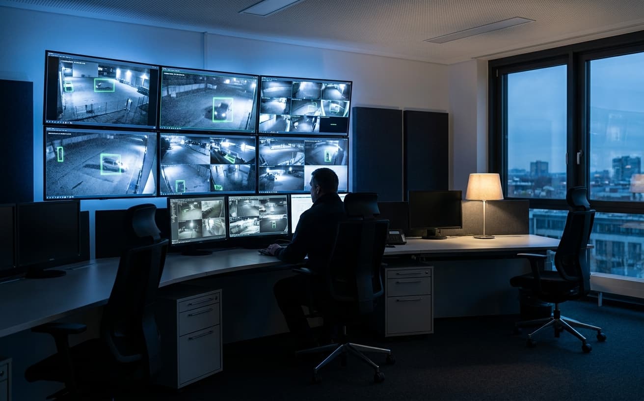
The first pattern is the fixed mast with multi-sensor head. Four to six cameras around a central pole, ten to twelve metres elevated, with on-board processing and a cellular uplink. The mast is positioned to cover defined zones. Detection happens at the edge. Alerts are filtered, classified, and pushed to a remote operator who confirms within seconds and triggers an audio challenge through a built-in loudspeaker. The intervention chain ends with a private security response or, in serious cases, the police. This pattern works well for sites with a defined footprint, predictable layouts, and a perimeter that can be observed from a small number of high points. Most urban infill sites fall into this category.

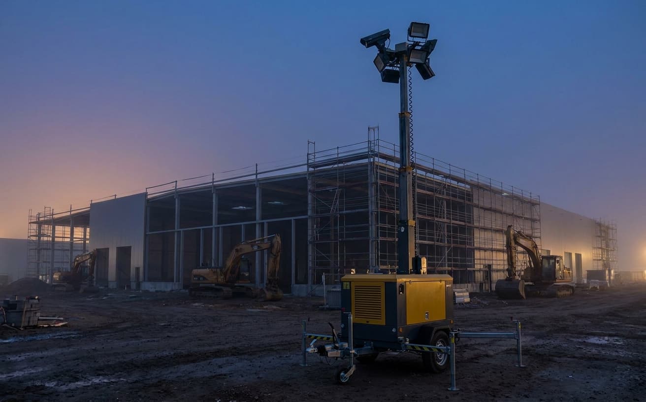
The second pattern is the mobile tower with the same sensor stack, repositioned as the site evolves. Construction sites are not static. The lay-down yard moves, the staging area expands, the storage of high-value material shifts as trades come and go. A fixed mast that was correctly positioned in month one is poorly positioned in month four. The mobile tower addresses this through repositioning that takes one technician and one hour. The trade-off is power: the tower runs on hybrid solar with a generator backup, and the energy budget constrains the number of sensors and the duty cycle. For large, evolving sites with shifting risk geography, this pattern outperforms fixed installations even at higher unit cost.

The third pattern is the autonomous patrol robot, paired with fixed or mobile sensors. The robot adds two capabilities that masts cannot deliver: unpredictability of route, which defeats observers who have studied the site, and physical presence in zones that no fixed sensor covers from above. The robot is not a replacement for the mast. It is a complement. Sites that use robots without fixed coverage end up with gaps in the seconds during which the robot is in another quadrant. Sites that use masts without robots end up with predictable blind spots between mast positions. The combined pattern, which we describe at length in BOSWAU + KNAUER. From Building to Security Technology, is what most demanding industrial customers settle on once they have run a few quarters of operational data.

What the theft profiles look like in the data

A site that has been monitored continuously for twelve months produces a distribution of incidents that is more structured than most operators expect. Roughly half of all theft attempts on a typical urban site cluster between two and five in the morning, on Sunday and Monday nights, in weeks where deliveries of high-value material have been visible from the public road during the prior week. This is not opportunism. It is reconnaissance followed by execution.

The opportunistic category, which most operators assume is the dominant pattern, is in fact a minority of events on monitored sites, though it remains the dominant pattern on unmonitored sites. The arithmetic is simple. Opportunism is deterred by visible technology and by the audio challenge. What remains, on sites that have visible deterrence in place, is the prepared theft. The prepared theft requires a different response: not deterrence, which has already failed at the point of detection, but speed of intervention.

The third profile, organised theft with vehicle and tools, is rarer in absolute numbers but accounts for the largest losses. These events are visible in the data because they show a pattern of pre-visit observation, sometimes from a vehicle parked at distance and recorded by the perimeter cameras days before the event. Sites that review their footage for these pre-visit patterns develop a defensive posture that fixed-camera-and-react deployments cannot match. The NICB and comparable trade bodies in Europe have published estimates that put organised construction theft losses in the high single-digit billions annually across the continent, which is the order of magnitude that justifies the investment in detection systems that look at the days before the theft, not only the minutes during it.

Integration with what is already on site

Most sites of any scale already have cameras. The cameras are usually consumer-grade or low-end commercial, recording to a local NVR, with no analytics layer and no intervention chain. Operators who consider a computer vision deployment frequently ask whether the existing cameras can be reused. The honest answer is sometimes, with limits.

Existing cameras can feed a centralised analytics platform if they support a standard streaming protocol, typically RTSP, and if their resolution and frame rate meet the model's minimum input requirements. The minimum for reliable detection of persons at twenty to thirty metres is around two megapixels and fifteen frames per second. Many installed cameras meet this. Where they fall short is night performance, weatherproofing for long-term mast mounting, and the field of view needed for wide-area coverage. The integration architecture that works in practice is a hybrid: existing cameras are kept for zone coverage and forensic recording, and new sensors are added for the active detection layer. The analytics platform reads both streams and applies a uniform classification model to all of them.

The second integration question is the alert pipeline. A detection that ends in an email is not a security event. A detection that ends in a confirmed operator response within sixty seconds is. Sites that have invested in computer vision without redesigning the alert pipeline end up with intelligent cameras and unintelligent responses, which produces the same losses as before at higher cost. The IEC 62443 and ISO 27001 frameworks have useful structures for thinking about the response chain, even though they were not written for construction. The frameworks force the question of who is on the other end of the alert, what they are authorised to do, and how their action is documented.

The third integration question concerns existing security service providers. Many sites already have a guarding contract. The serious operators do not terminate that contract when they install computer vision. They restructure it. The guard moves from continuous patrol, which is the most expensive and least effective use of human attention, to a verification and response role. The computer vision system generates the events. The guard verifies and responds. The number of guards needed falls. The effectiveness of the guards who remain rises. This is the operational model that produces both cost reduction and loss reduction in the same deployment, and it is the model that ASIS International has been describing as the industry direction for some time.

Latency, false positives, and the operator's actual experience

Two numbers determine whether a deployment works in daily operation. The first is end-to-end latency, from event in the field to alert on the operator's screen. The second is the false-positive rate per camera per twenty-four hours.

End-to-end latency in a properly designed system runs between one and three seconds. The detection runs at the edge, the classification completes in under five hundred milliseconds, the alert is pushed through a cellular or fibre link, and the operator's screen updates. Systems that route detection through a distant cloud add latency that the field cannot afford. A six-second latency sounds small in a meeting room. On a site, six seconds is the difference between an audio challenge that interrupts the theft and an audio challenge that addresses an empty space.

The false-positive rate is the variable that determines whether the operator pays attention to the system or learns to ignore it. The benchmark for a usable deployment is below five false positives per camera per day in stable conditions. Above that, operator fatigue sets in, and within weeks the response time degrades to the point where the system is operationally inactive even though it is technically running. Sites that do not measure this number end up surprised by their own outcomes. Sites that do measure it use the number as the primary tuning target for the first three months after installation. The model is retrained on site-specific data, the geofences are adjusted, the time-of-day filters are refined, and the rate falls.

The combination of latency and false-positive control is what separates a system that produces measurable outcomes from a system that produces dashboards. CISA and NIST CSF 2.0 both, in their respective contexts, emphasise the operational measurement of detection systems over their nominal capability. The same principle applies here. A camera that can detect a person is not a security system. A camera that detects a person, classifies the event correctly, and triggers a verified response within seconds, with a false-positive rate that the operator can live with, is.

What holds

Computer vision against construction site theft works when it is deployed as a chain, not as a component. The chain runs from sensor to model to alert to operator to response to documentation. Each link has measurable properties. Each link is the responsibility of a named party. The links that are skipped are the ones that produce the failures, and the failures are usually attributed to the wrong link in the post-mortem. The camera gets blamed for what the response chain failed to deliver.

The operators who get this right share three habits. They measure their losses before they buy. They define their success metrics before they install. And they review their own data quarterly, not annually, because the threat picture moves faster than the budget cycle. The systems that look impressive in a sales demonstration are not always the same systems that look impressive in the twelfth month of operation. The two views can be reconciled only by data from the site itself.

For operators who want to test these claims against their own situation without committing to a long procurement process, the appropriate entry point is Path II, the three to five day audit. The audit produces a written deliverable with a schedule of vulnerabilities, an incident reconstruction for the prior twenty-four months where records permit, and a comparative economic case across status quo, partial modernisation, and full platform deployment. What the operator does with the deliverable is the operator's decision. The audit is not a sales mechanism. It is a basis for the next decision, which may or may not involve us.

Frequently asked questions

How effective is computer vision against construction theft?

Effectiveness is measured against a baseline, not in absolute terms. On sites that move from unmonitored or traditionally guarded to a multi-sensor computer vision deployment with an active response chain, the typical reduction in successful theft events sits between sixty and eighty-five percent in the first twelve months, depending on the threat profile and the response time achievable on the site. The reduction is steeper for opportunistic theft and shallower for organised theft with vehicle support. The data behind these ranges comes from operator-reported figures and industry sources such as the GDV in Germany.

Which theft patterns are detected most reliably?

Perimeter breach by persons on foot, vehicle approach to restricted zones, and loitering above a defined time threshold are the patterns with the highest detection reliability, generally above ninety-five percent in good visibility. After-hours presence in defined high-value zones, such as the lay-down area for copper or finished electrical components, also detects reliably. The patterns that are harder are tool-specific identification at distance, intent inference from a single behavioural signal, and theft by personnel with legitimate site access. The last category requires access control integration, not vision alone.

How is the system integrated with existing CCTV?

Existing cameras that support standard streaming protocols and meet minimum resolution and frame rate thresholds can be incorporated into the analytics layer alongside new sensors. The integration runs at the platform level, where a uniform classification model reads all streams. Cameras that fall below the thresholds remain useful for forensic recording but are supplemented with new sensors for active detection. The alert pipeline is redesigned around the combined sensor set, and the existing guarding contract is typically restructured to a verification and response role rather than continuous patrol.

What is the typical detection latency?

End-to-end latency, from event in the field to alert on the operator's screen, runs between one and three seconds in a properly designed system with edge processing and a direct cellular or fibre uplink. Systems that route classification through distant cloud infrastructure add latency that the operational context cannot absorb. The audio challenge to the intruder, which is the active deterrence element, fires within the same window. Latency above five seconds materially degrades the deterrence value, because the intruder is no longer in the same position when the response arrives.